How to use MS Excel conditional formatting to change text/background colors of cells automatically

When doing some Excel-based marketing report, whether it’s web analytic report or sales related report, most of the times, I used some conditional formatting to automatically highlight cells that meet certain criteria such as highlighting cells of under-performing or over-performing shops, under/over-performing regions for revenue reports; highlighting cells based on contract value; highlighting cells that have “N/A” or negative numbers; or highlighting cells of web pages that have poor performance in page visits for a certain period of time.
If your spreadsheet is short, you may not need to to perform conditional formatting since you can just manually check each cell in certain column and row; however, you shouldn’t waste much time doing it, especially when Excel provides an easy way for you to do it quickly and automatically.
Conditional formatting
Conditional Formatting is a function that allow user to set “alerts” based on values contained within cells. Basically, you can set criteria for the data set and then define the format of the cells. You can define your own rule or use Excel pre-defined conditional rules.
Pre-Defined Conditional Formatting Rules
To enable conditional formatting, select the range of cells that should be referenced -> click the Home tab -> click the Conditional Formatting button on the menu ribbon.
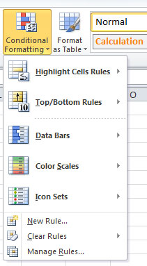
Excel has some pre-configured options that are pretty simple and straight-forward to use such as Highlight Cells Rules -> Greater Than (or Less Than, or Equal To, or Between, etc…). You can use one or more of these default options and be done right here.
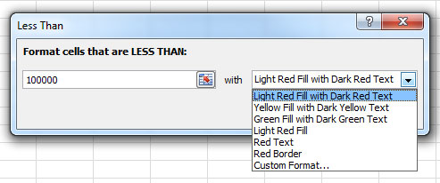
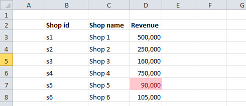
For example, we’ll going to highlight Shops that generated less than 100,000 in revenue. To do this, just mouseover Highlight Cells Rules -> Less Than, then enter 100,000 in the field -> Hit OK and see the result.
New Conditional Formatting Rules
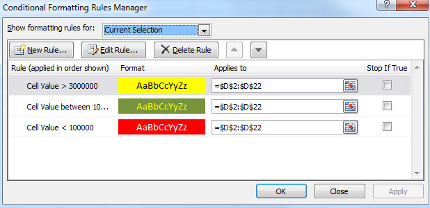
If you want to use different highlighting colors or have more complex conditional rules, you can create New Rule. For example, we will define the following criteria for the Conditional formatting
- Shop with revenue < $ 1,000,000 : Red background, white text
- Shop with revenue between $ 1,000,000 – $ 3,000,000 : Green background, white text
- Shop with revenue > $ 3,000,000 : Yellow background, black text
- First, let’s clear any rules that are there by clicking the Home tab -> Conditional Formatting -> Clear Rules. Then repeat the steps above: Select the range of cell -> Home tab -> Conditional Formatting -> New Rule to start create a new rule.
- Use the Format Only Cells That Contain option -> Cell value -> Less Than -> 1,000,000
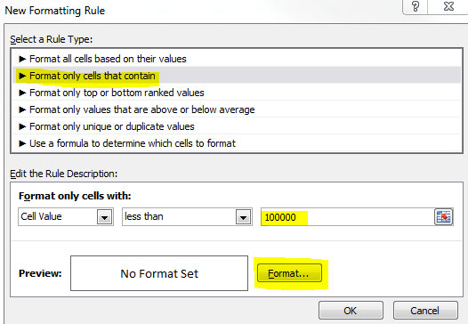
- Click the Format button to specify the font color (white), and the fill color (red). Hit OK to save and done with the first condition.
- Repeat the steps above to add the 2nd and 3rd rules. You can also edit the rules, including adding and deleting, by clicking the Home tab -> Conditional Formatting -> Manage Rules
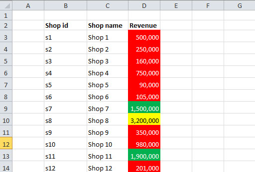
Final results:
How about a post about doing Conditional Formating by using script? You should cover it, too.